はじめに #
NumPyで利用できる数学の関数について。
mathライブラリの数学の関数は一般にスカラー値にしか適用できない。一方、NumPyの数学の関数はスカラー値に加え、リストやnumpy.arrayオブジェクトにも適用できる。
環境 #
- NumPy 1.19
三角関数・逆三角関数 #
角度の単位はラジアン。
| 関数 | 記法 | 説明 |
|---|---|---|
| sin | np.sin(a) | |
| cos | np.cos(a) | |
| tan | np.tan(a) | |
| arcsin | np.arcsin(a) | |
| arccos | np.arccos(a) | |
| arctan | np.arctan(a) | 戻り値の範囲は[-pi/2, pi/2] |
| arctan2 | np.arctan2(a, b) | a/bのarctanを返す。戻り値の範囲は[-pi, pi] |
>>> import numpy as np
>>> a = np.array([0, np.pi/6, np.pi/3, np.pi/2]) # np.piは円周率
>>> b = np.sin(a)
>>> b
array([ 0.       ,  0.5      ,  0.8660254,  1.       ])
>>> np.arcsin(b)
array([ 0.        ,  0.52359878,  1.04719755,  1.57079633])
>>> np.deg2rad([0, 90, 180])         # degからradへ変換
array([ 0.        ,  1.57079633,  3.14159265])
>>> np.rad2deg([0, np.pi/2, np.pi])  # radからdegへ変換
array([   0.,   90.,  180.])
三角関数・逆三角関数のグラフは以下の通り。
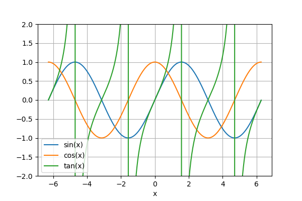
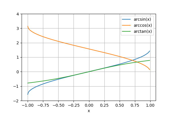
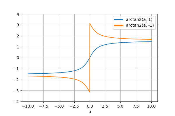
以下のコードで描画した。
import numpy as np
import matplotlib.pyplot as plt

x1 = np.arange(-2*np.pi, 2*np.pi, 0.01)

fig, ax = plt.subplots()
ax.plot(x1, np.sin(x1), label="sin(x)")
ax.plot(x1, np.cos(x1), label="cos(x)")
ax.plot(x1, np.tan(x1), label="tan(x)")
ax.set_ylim(-2, 2)
ax.set_xlabel("x")
ax.grid(); ax.legend()
plt.show()

x2 = np.arange(-1, 1, 0.01)

fig, ax = plt.subplots()
ax.plot(x2, np.arcsin(x2), label="arcsin(x)")
ax.plot(x2, np.arccos(x2), label="arccos(x)")
ax.plot(x2, np.arctan(x2), label="arctan(x)")
ax.set_ylim(-2, 4)
ax.set_xlabel("x")
ax.grid(); ax.legend()
plt.show()

a = np.arange(-10, 10, 0.01)
b1, b2 = 1, -1

fig, ax = plt.subplots()
ax.plot(a, np.arctan2(a, b1), label="arctan2(a, 1)")
ax.plot(a, np.arctan2(a, b2), label="arctan2(a, -1)")
ax.set_ylim(-4, 4)
ax.set_xlabel("a")
ax.grid(); ax.legend()
plt.show()
双曲線関数 #
| 関数 | 記法 |
|---|---|
| sinh | np.sinh(a) |
| cosh | np.cosh(a) |
| tanh | np.tanh(a) |
| arcsinh | np.arcsinh(a) |
| arccosh | np.arccosh(a) |
| arctanh | np.arctanh(a) |
端数処理 #
| 記法 | 説明 | |
|---|---|---|
| 四捨五入 | np.around(a, decimals=0) | 10^(-decimals)の1つ下の位を四捨五入 |
| 四捨五入 | np.round_(a, decimals=0) | aroundと同じ |
| 0方向への丸め | np.fix(a) | |
| 負方向への丸め(切捨て) | np.floor(a) | |
| 正方向への丸め(切上げ) | np.ceil(a) | |
| 0方向への丸め | np.trunc(a) |
>>> np.around(123.456, decimals=0)   # 0.1の位を四捨五入
123.0
>>> np.around(123.456, decimals=1)   # 0.01の位を四捨五入
123.5
>>> np.around(123.456, decimals=-2)  # 10の位を四捨五入
100.0
>>> np.fix([0.7, 3.2, -0.7, -3.2])   # 0方向への丸め
array([ 0.,  3., -0., -3.])
>>> np.floor([0.7, 3.2, -0.7, -3.2]) # 負方向への丸め
array([ 0.,  3., -1., -4.])
>>> np.ceil([0.7, 3.2, -0.7, -3.2])  # 正方向への丸め
array([ 1.,  4., -0., -3.])
>>> np.trunc([0.7, 3.2, -0.7, -3.2]) # 0方向への丸め
array([ 0.,  3., -0., -3.])
和・積・差分 #
1つの配列に含まれる要素の和・積・差分。
>>> a = np.array([[1, 2], [3, 4]])
>>> np.sum(a)          # 全要素の和
10
>>> np.sum(a, axis=0)  # 列方向の和
array([4, 6])
>>> np.sum(a, axis=1)  # 行方向の和
array([3, 7])
>>> np.prod(a)         # 全要素の積
24
>>> np.prod(a, axis=0) # 列方向の積
array([3, 8])
>>> np.prod(a, axis=1) # 行方向の積
array([ 2, 12])
>>> b = np.array([[1, 2, 4, 8], [3, 5, 9, 7]])
>>> np.diff(b)         # 最大の軸方向(axis=1)の差分
array([[ 1,  2,  4],
       [ 2,  4, -2]])
>>> np.diff(b, axis=0) # 列方向の差分
array([[ 2,  3,  5, -1]])
>>> np.diff(b, n=2)    # n: 差分をとる回数( =np.diff(np.diff(b)) )
array([[ 1,  2],
       [ 2, -6]])
指数関数・対数関数 #
>>> np.exp([0, 1])         # 指数関数
array([ 1.        ,  2.71828183])
>>> np.log([1, np.e])      # 自然対数
array([ 0.,  1.])
>>> np.log10([1, 10, 100]) # 常用対数
array([ 0.,  1.,  2.])
その他 #
>>> np.sqrt([1, 4, 9])          # 平方根
array([ 1.,  2.,  3.])
>>> np.cbrt([1, 8, 27])         # 立方根(三乗根)
array([ 1.,  2.,  3.])
>>> np.square([1, 2, 3])        # 二乗
array([1, 4, 9], dtype=int32)
>>> np.absolute([-3, -1, 1, 3]) # 絶対値
array([3, 1, 1, 3])
>>> np.sign([-3, -1, 1, 3])     # 符号
array([-1, -1,  1,  1])
>>> np.maximum([-3, -1, 1, 3], [4, 2, -2, -4]) # 各要素の最大値
array([4, 2, 1, 3])
>>> np.minimum([-3, -1, 1, 3], [4, 2, -2, -4]) # 各要素の最小値
array([-3, -1, -2, -4])
1つの配列の最大値・最小値を求める場合は、np.max, np.min関数を使う。